How coordinates (latitude and longitude) impact price prediction in real state

Analyzing results for different regression algorithms during house price prediction, we found huge improvement by incluidng latitude and longitude values as feaures for the model. Let’s review and compare some of the results obtained.

• Data belongs to Colombian real state market
• Some of the main features used are:
  • Number of rooms
  • Number of garages
  • Number of bathrooms
  • Stratum (Value from 1 to 6 which provides socio-deographics information of the area)
  • Type of property
  • Age of the property
  • Size of the property
  • Geographic location of the property
  • Price of property (which is the target feature)

Data Exploratory

For data exploratory analysis we choose Rapidminer Studio. Let’s perform some basic EDA for the most important characteristics of the data to be used.

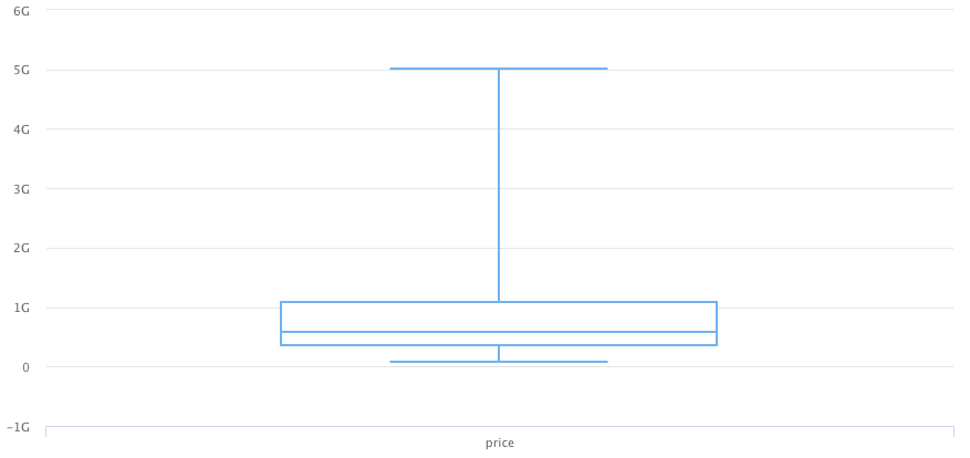
The current dataset belongs to properties from Colombia. As we can see in next plot, most of the samples are contained between 350M and 1000M

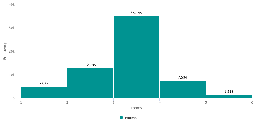
Number of rooms is contained between 1 and 5.

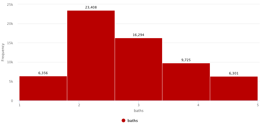
Number of bathrooms is within 1 and 5, same as number of rooms.

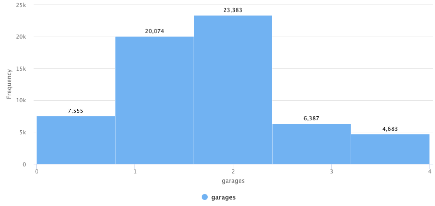
Number of garages is between 0 and 4.

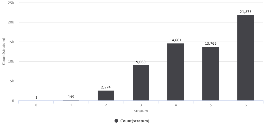
The “stratum” feature helps to provide a socio-demographic idea of the area where the property is located. Range is from 1 to 6, where 1 is low income area and 6 is high income area.

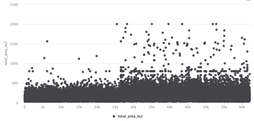
Another important feature is area of the property. This plot shows a lot of outliers that require treatment.

Data definition

Based on previous basic analysis, we have defined following filters in order to get a model more accurate.

• Stratum equals to 4. Other stratum requires to consider more features to get more accuracy on the model. After the filter is applied, this column is useless so it will be dropped.
• Price below 600M. For Stratum 4, 600M is a good thresholds to discard outliers.
• Total area in square meters is maximum 180. Same as price, for stratum 4, 180 square meters is a good threshold to discard outliers.
• For the price we applied a range reduction in order to change from millions to thousands by dividing all rows by 1M.

Since we are using pandas to load the data in tabular form, we use dataframe functions to filter the data.

In order to get how much improvement is reached by using coordinates, we have defined 2 filters and performed model training for each filter.

Filter 1: Without coordinates

{
    df['price'] = data['price']/1000000
    df = df[df['stratum'] == 4]
    df = df[df['price'] <= 600]
    df = df[df['total_area_m2'] == 180]
    df.drop('stratum', axis=1, inplace=True)
}

Filter 2: Coordinates for Colombia Capital (Bogota)

{
    df['price'] = data['price']/1000000
    df = df[df['stratum'] == 4]
    df = df[df['price'] <= 600]
    df = df[df['total_area_m2'] == 180]
    df = df[df['lat'] <= 4.8]
    df = df[df['lat'] >= 4.6]
    df = df[df['lng'] <= -74.2]
    df = df[df['lng'] >= -74.0]
    df.drop('stratum', axis=1, inplace=True)
}

Model Training

In order to apply different hiperparameters for all the regressions (since we are predicting a price, the model training must be a regression) functions selected, we have prepared different functions for each model with several parameters.

The best parameters for each model will be selected and the results along with the configuration will be appended to a dataframe to compare the results.

    results = results.append(linear_regression(x_train, y_train, x_test, y_test), ignore_index=True)
    results = results.append(ransac(x_train, y_train, x_test, y_test), ignore_index=True)
    results = results.append(ridge(x_train, y_train, x_test, y_test), ignore_index=True)
    results = results.append(elasticnet(x_train, y_train, x_test, y_test), ignore_index=True)
    results = results.append(linearsvr(x_train, y_train, x_test, y_test), ignore_index=True)
    results = results.append(bayesianridge(x_train, y_train, x_test, y_test), ignore_index=True)
    results = results.append(lasso(x_train, y_train, x_test, y_test), ignore_index=True)
    results = results.append(decisiontree_regressor(x_train, y_train, x_test, y_test), ignore_index=True)
    results = results.append(randomforest_regressor(x_train, y_train, x_test, y_test), ignore_index=True)
    results = results.append(gradientboost_regressor(x_train, y_train, x_test, y_test), ignore_index=True)
    results = results.append(sgd_regressor(x_train, y_train, x_test, y_test), ignore_index=True)
    results = results.append(huber_regressor(x_train, y_train, x_test, y_test), ignore_index=True)
    results = results.append(theilsen_regressor(x_train, y_train, x_test, y_test), ignore_index=True)
    results = results.append(xgboost(x_train, y_train, x_test, y_test), ignore_index=True)

Model Evaluation

During training model, we splitted the data with 80% used for training and 20% for testing. RMSE is used to compare the accurateness of the models. Basically we get the RMSE between the price predicted and real price from the testing dataset.

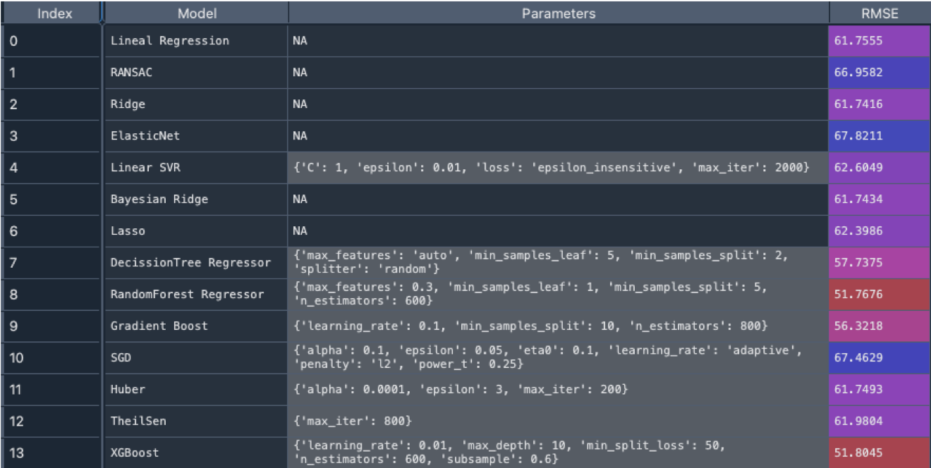
Best results are obtained for XGBoost, Random Forest Regressor, Gradient Boost, Decission Tree Regressor etc. In the case of data from filter 1 (Without coordinates) the best RMSE is 51.8M

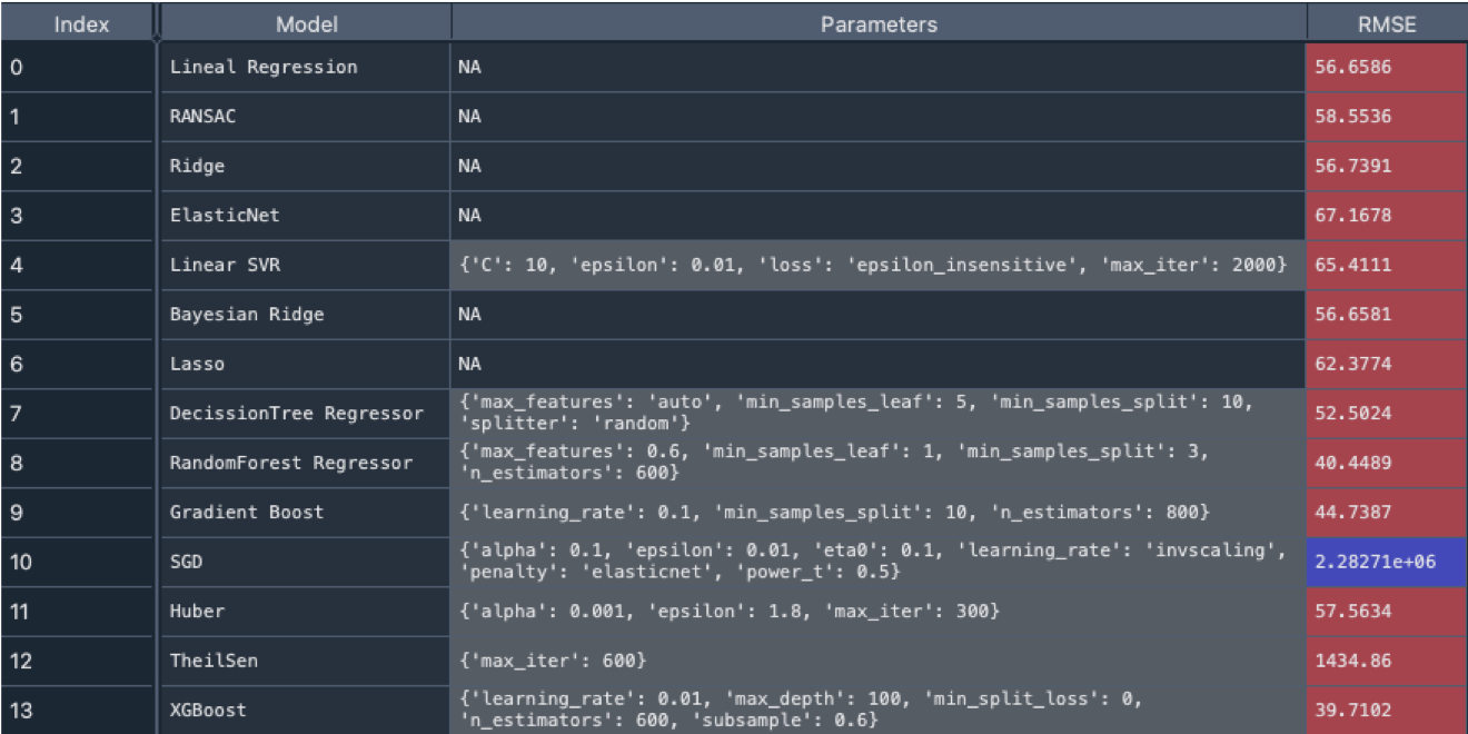
For filter 2 (including coordinates in the dataset), the improvement is high, with a reduction of 12M in RMSE. XGBoost and Random Forest continues to be the best model reaching a RMSE of 39.7M

Final Thoughts

As we can see, the coordinates can be a very important feature (as it was supposed, since it is well know that real state is all about location, location, location) to consider in house prediction.

In additional testing, we have found some additional insights that we can consider in order to improve the accuracy of house pricing models.

• Continue to add more data. I have been feeding my dataset with additional data and always getting small improvements in the results.
• Consider more features such as: Security in the area, quality of schools nearby, parks/malls/stores nearby, accessibility, noise levels etc.
• Historical data regarding sales of each property
• Real state market indicators